Pushing the boundaries in Remote Sensing for crop classification
Welcome back to the second part of our exciting journey into Remote Sensing and agricultural applications! In the first part, we discussed how to start any Machine Learning project, with a closer look at crop classification specifically. We showed that a Transformer model significantly outperforms traditional statistical models and their deep-learning peers.
In this second part of the blog post series, we will go deeper into the model optimization process, covering everything from data augmentation to post-calibration of our Transformer model. We'll also discuss our exploration into training stability and how to handle the inevitable noise in Remote Sensing data. Let's dive right in!
Looking back: insights and discoveries from part 1
In the first part of this series, we started by highlighting the importance of crop classification for agriculture, particularly its role in supporting the European Union's Common Agricultural Policy and promoting sustainable practices. We also addressed the complexities of this task, mainly due to variations in data accessibility and labelling inconsistencies across different countries.
We created a pixel-based crop classification model to address these challenges, investigating the benefits of pixel-based approaches and time series analysis on multispectral data. Our first approach was to get a baseline with simple statistical models, where a LightGBM model proved to perform best. We then dived into custom deep learning architectures, comparing the baseline with models like CNN, LSTM, and Transformer.
The Transformer model came out on top, having the best performance for every single class. In the second part of our journey, we'll continue refining our Transformer model, exploring various techniques to enhance the model's performance.
Establishing consistency: examining the stability of model training
As we started to refine our Transformer model, we first checked the stability of the model's training process. The stochastic nature of machine learning training introduces variations in model performance across different runs, even when the hyperparameters remain unchanged. These variations could mislead us into attributing performance improvements to our refinements when they result from this inherent stochasticity.
To counter this, we put together a stable training setup. We regulated the training environment, guaranteeing that the model and training approach stayed the same across different training runs. The model hyperparameters were left unchanged, with its initialization happening randomly. The dataset splits (training, validation, and testing) were the same over different model runs, but we kept the random sampling of this data during training.
We ran the training five times, resulting in five different models. The graph below shows the difference in evaluation results between the worst models. The dashed horizontal line shows the worst and best macro F1 performance (class-level average), whereas the bars show each class's worst and best performance. The average macro F1-score over the five model runs equalled 75.3%.
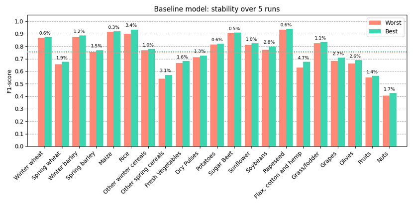
Visual representation of the best and worst class-specific performances across five model iterations.
The results from the image above show us that training happens fairly stable, with a minor change in macro F1-score between the worst and best model run (1.02% difference). Also, each crop class' performance mostly stayed the same over the different runs. This slight variation in performance speaks to the robustness of our Transformer model. It sets the stage for our upcoming series of experiments, where we investigate the influence of data augmentation, noise reduction, and more. This stability experiment assures us that any notable change in performance is likely due to model or training refinements and not merely the product of the training's inherent randomness.
Data augmentation: the easiest way to enhance model performance
After confirming the training’s stability, we started refining our model. The first step was data augmentation. This common strategy in machine learning helps reduce overfitting and makes your model more robust and thus can yield better performance. For us, the reason to go for data augmentation was two-fold. On the one hand, we were dealing with limited data for some classes, so we wanted to generate more artificial data. On the other hand, we discovered that the model was sensitive to a variance in seasonality, which we can reduce through augmentation.
We applied several data augmentation techniques to our model. Each augmentation aims to add minor changes in the input signal without affecting the target labels (crop classes). The augmentations that yielded the best results were:
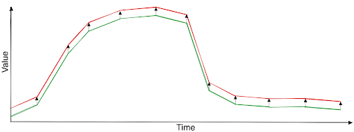
- To shift the whole time series across all the bands up or down for a specific offset. This prevents the model from overfitting particular values in the time series and helps the model to focus on the evolution of the spectral bands over time.
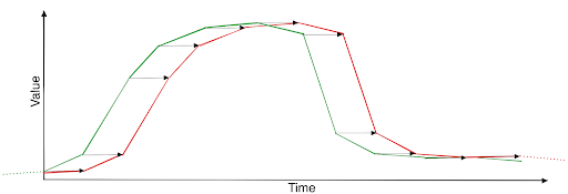
- To shift the whole time series left or right with one time-step at most. Training with this augmentation improved the robustness of the model with a slight variance in seasonality, which was a problem present in older models that we discovered through error analysis.
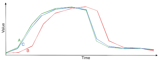
- Merging two series through linear interpolation, given they belong to the same target class. Say we have two series of the same class, A and B. For this augmentation, we would keep the majority of series A (e.g. 90%) and take the remaining (10%) from series B to get to a fictive series C. By augmenting this way; we create fictive samples which belong to the provided crop class. Note that this assumes clean data and that all series of the same class show similar characteristics.
The augmentations were applied randomly, where none or sometimes even all of them were used. The graph below shows the result after adding this mechanism for stochastic augmentations. Overall, the performance increases with a macro F1-score of 2.2%. However, the most notable is that almost all classes benefit from these augmentations, with the ones that performed the worst increasing the most in performance. This improvement shows that data augmentation, or manipulating an existing dataset carefully, can substantially enhance a model’s performance.
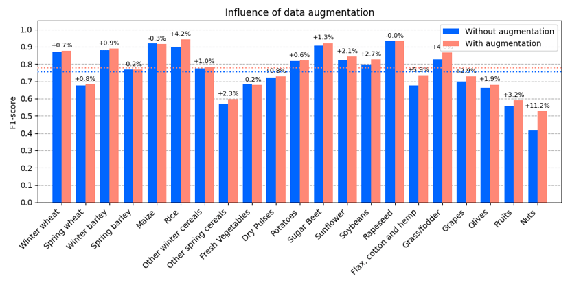 Visualization of significant performance enhancement across all classes, particularly those initially underperforming, following the introduction of stochastic data augmentations.
Dealing with noise: cleaning up for clearer insights
Next, we tackled the influence noise has on the performance of our model. Noise, often resulting from clouds, snow, or even sensor errors in Remote Sensing, can distort the signal and create challenges for our model's training, affecting its performance. Note that the models discussed before already operated on cleaned data, so this section analyzes the opposite: what would happen if we didn't clean the input signals?
Several techniques are applied to clean the data, wich was done by the domain experts at VITO. Among these processing steps, the following had the biggest impact:
- Temporal compositing to minimize the impact of temporary effects like cloud cover, atmospheric variations, and sensor noise. we aggregate all available signals at a consistent frequency of 10 days.
- Masking out clouds and snow so that the input represents measures done directly on the agricultural field of interest.
- Linearly interpolating gaps in the time series, introduced by the masking from the previous step.
- Erode (or cut away) the sides of the known agricultural fields. This helps us get a cleaner signal, where we remove noisy signals found at the border of a field that may overlap with other land due to the lower (10m) resolution of sentinel-2.
- Cluster neighboring pixels from a single field and take this cluster’s median value. This helps to eliminate noise present within one field.
The following two images visualize the result of this cleaning. The former image shows a raw observation, whereas the latter shows the processed result.
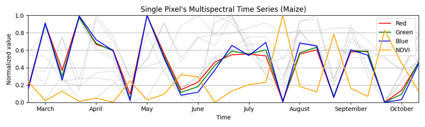
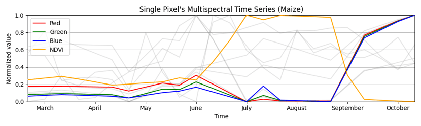
Contrast between raw observations and processed, noise-reduced data, highlighting the effectiveness of expert cleaning techniques in Remote Sensing applications.
To measure the impact of noise, we ran the model on raw data and compared its performance with that on data where we had carefully minimized noise. The bar chart below shows the results, showing a significant performance boost from cleaning the data. The overall improvement is 2.6% in the Macro F1-score. Also interesting to note is that the influence of noise reduction is equally spread across the crop classes, with no single class suffering significantly more from the noise. The lesson is clear: cleaner signals lead to better model performance. Minimizing noise in our data makes it easier for the model to learn underlying patterns and classify crops more accurately. Despite that, it's still interesting to see how well a transformer model can deal with such noisy signals, still obtaining a decent result when operating on very noisy data.
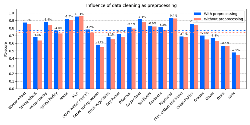
Comparison of model performance on raw data versus noise-reduced data, demonstrating a significant, evenly distributed performance boost across crop classes upon data cleaning.
Unveiling the power of transformers: deriving expert indices automatically
In the world of Remote Sensing, experts often use indices such as the Normalized Difference Vegetation Index (NDVI) to extract valuable information from the data. But why is that? The reason lies in the unique ability of these indices to combine different inputs, usually by linearly combining various bands, to highlight specific features of the landscape, like vegetation health in the case of NDVI.
These expert indices have been handy tools. However, with the advent of deep learning models, things are beginning to change. Specifically, our Transformer model displayed an impressive ability to derive these indices on its own, without having them explicitly listed as inputs. This capability is a testament to the power of the Transformer's self-learning and its potential to identify and leverage critical features in the data independently.
We tried providing the model with and without these expert indices in our experiments. The surprising finding was that the two setups had no significant performance difference. It became evident that our model, like a diligent student, was efficiently doing its homework and deriving these indices by itself when necessary.
The following graph shows three different scenarios. Note that all three of the models use Sentinel-1 and METEO data supplementary. The different models had the following additional inputs:
- An optical-only model: sentinel-2 bands 2 to 8, and 11 and 12.
- A model using only expert indices: NDVI, NDMI, NDWI, NDGI, NDTI, ANIR, NDRE1, NDRE2, NDRE5.
- A model using both the optical bands as the expert indices as inputs.
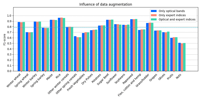
Comparison of model performance using different input scenarios: optical-only data, expert indices only, and a combination of both, illustrating a similar macro F1-score across all three setups.
As shown in the image, all three models perform very similarly, with a macro F1-score of 78.5% for the optical-only model, 78.5% for the expert indices-only model, and 78.6% for the model using both in its inputs. Despite that this experiment did not yield any performance improvements, it was still an interesting experiment to conduct since it provides insights into the reasoning capabilities of modern Deep Learning methods.
A suite of experiments: trying out various techniques
Seeking to enhance our model's performance further, we underwent a series of additional experiments. Even though our default values often proved to be the most effective, these explorations still provided us with valuable insights. Nonetheless, they can be a source of inspiration to you to improve your own models. The experiments we did are the following:
- Adjusting Transformer sizes showed that four layers, eight heads, and an embedding size of 128 worked best; larger sizes didn't notably improve performance and increased training and inference times.
- Various optimizers and learning rates were tested, with Adam and an initial learning rate of 1e-3 proving most effective; SGD notably underperformed in comparison.
- We tried different loss functions; the default, focal loss based on cross-entropy, marginally outperformed alternatives like simple cross-entropy and mean squared error (MSE).
- We experimented with different learning rate schedules, where gradually reducing on a loss plateau proved to be the best scheduler for our use case.
- Testing dropout influence showed no clear impact on evaluation results, but it did help lower training scores, indicating a potential reduction in overfitting.
- We made a comparison between different activation functions like ReLU, GeLU, and LeakyReLU; the default activation, ReLU, performed on par with alternatives, confirming its suitability for our model.
These additional experiments provided valuable insights and directions, verifying our design decisions when creating the model. Despite not leading to significant improvements, these experiments played a crucial role in the process, solidifying our understanding of the model's functioning and helping us rule out less effective alternatives. With these extensive investigations, we feel confident about our choices and the final model's robustness.
Reflecting on our journey: the final model results
After a rigorous and iterative journey of experiments, we arrived at the final model. This model emerged through careful refinement and critical decision-making, significantly improving our original model. From maintaining training stability, applying strategic data augmentation, meticulously dealing with data noise, and acknowledging the capability of deep learning in deducing expert indices, each step helped shape our model to its optimal state.
The final model outperformed the initial model across all parameters, showing a robust overall improvement. The following graph shows the difference in performance between the baseline model, obtained at the end of part one of this blog series, and the final model we have now. We trained five models for both model versions to reduce the variance in performance obtained after multiple model runs. Overall, the model's performance improved by 4.16% in macro F1, going from 75.29% to 79.45%.
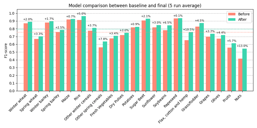
Performance comparison between the initial baseline model and the final optimized model, demonstrating a notable increase of 4.16% in macro F1 score.
One of the most gratifying moments in this project has been seeing the real-world performance of our model. The image below shows how our model operates in a real-life scenario, successfully distinguishing between various crop types. In the end, these results underline the success of our model and, more importantly, the effectiveness of the methodology we adopted for this project. This thorough experimentation and model refinement approach allowed us to create a robust and reliable tool, ready to take on real-world challenges in Remote Sensing.

Visualization of the model's real-world performance in accurately distinguishing between various crop types.
Exploiting global uncertainty: model post-calibration
As a final touch to our best-performing model, we added post-training calibration. One of the reasons to calibrate a model is if you want to extract global counts from it. To help illustrate this, let's give an example; say you want to get the distribution of crops that grow in Europe.
One way to calculate this is to use our crop classification model to predict the crop types for all European fields. Given that we trained this model to be a good crop classifier, combining its prediction to get a crop distribution estimate makes sense. However, this does not take the certainty of each prediction into account. Alternatively, we can use the probability of each prediction to create this global distribution, but this might be wrong since the model was not explicitly trained to reflect uncertainty in its predictions. If our model is slightly overconfident, a 90% probability does not mean it's correct 90% of the time; it's less often correct than that.
A better way to approach this challenge is to calibrate your model first. This is done after the model's training and aims better to reflect a prediction's certainty regarding its probability. Model calibration is an active research topic and would bring us too far in this blog post. For those interested, this paper gives an excellent overview of different calibration methods.
To calibrate our model, we employed temperature scaling, an effective method for calibrating predictive distributions in machine learning models. This calibration technique aims to provide better probability estimates for our predictions without sacrificing performance (fun fact, we even gained 0.6% in macro F1-score!). The image below is called a calibration plot, which shows the alignment of the model's prediction probabilities with the actual accuracy. Note that we calibrate the model using the validation dataset, where the calibration results are measured using the test dataset.
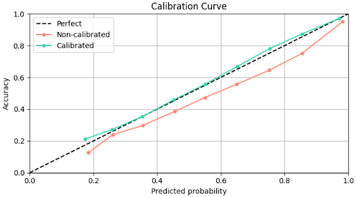
Calibration plot demonstrating the alignment of model's prediction probabilities with actual accuracy after employing temperature scaling.
For our use case, where we aim to count the number of crop fields across Europe, a suitable metric is to compute the relative count regarding the actual count. By doing so, we can see how far off the model's predicted count is and if the model is over- or underestimating. Below is a visual depiction of the calibration effects at the class level, providing a clear comparison of the model's performance pre- and post-calibration. What is also interesting to see is that the model's count accuracy gets worse the worse its classification performance is, indicating a high uncertainty for these classes. In essence, post-calibration preserved our model's performance and enhanced its practical utility for the crop counting use case. This step illustrates the value of considering the end application when optimizing and refining machine learning models.
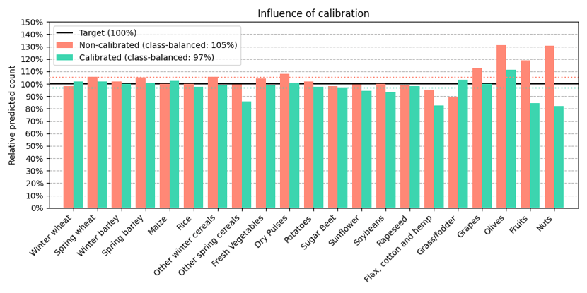
Visual representation of the significant reduction in Mean Absolute Error for each crop type after applying temperature scaling.
Advancing sustainability in Remote Sensing applications: a journey of continuous improvement
In the second part of this blog series, we've continued to harness the power and versatility of Transformer models for pixel-level crop classification, building upon the strides made in the first part. Our focus shifted from identifying an effective solution to continuously refining it, ensuring that our model evolves to meet the arising challenges present in Remote Sensing applications.
Our final model, though not perfect, represents a significant evolution from our baseline model. Its performance in real-world conditions shows the potential of Transformer models in Remote Sensing applications, promising a bright future. Next, we're excited to explore the potential of three-dimensional input instead of limiting our model to time series alone. We are already looking forward to what the future may hold!
Eager to share your thoughts or suggestions about our model? Leave a comment or contact me via LinkedIn!