How to forecast on timestamped tabular data: a fusion of both worlds

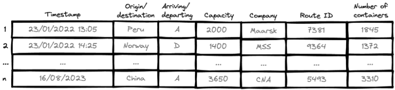
First things first, what is timestamped tabular data? To get a better understanding, let us look at the example figure below of ships arriving and departing from a port. Each entry/row represents an arriving or departing ship. It has a timestamp (obviously) and is characterized by a number of different properties.

Timestamped (tabular) data in such a format is omnipresent in this world and unlocks several valuable use cases:

• Demand forecasting: predicting customer demand for products or services, which benefits inventory management and production planning.
• Sales forecasting: a product of a particular category being sold at a given time at one of multiple possible shops (locations).
• Inventory forecasting: changing inventory levels of a particular raw material to prevent over-/understocking.
• Predictive maintenance: sensors registering temperature/vibrations/usage of a particular machine to estimate pre-emptively when to maintain it.
• Energy forecasting.
• Anywhere data is generated on the fly with different properties.

Timestamped tabular data is not a straightforward format. Due to the timestamps, there is a temporal relation that exists across rows, causing some rows to depend on others. Most popular modeling methods expect either pure tabular data (no cross-row relation), or pure univariate time series (timestamps + corresponding numeric values). Transforming the timestamped tabular data to a purely tabular format is suboptimal since the temporal dependency between rows is not modeled well. This technical blog post will dive into one of the ways such a problem can be tackled well. You will learn how to employ existing time series and tabular techniques, and fuse them together in order to not reinvent the wheel. Be warned, this article is not about benchmarking different methods against one another!

A supply chain example: cargo ships forecasting

Let’s retake the fictive example scenario from the introduction to make the problem more concrete. A port wants to know how many containers each given ship will have on board in the future (since the ship is exploited by a private company, the port doesn’t have access to that information). This is very valuable knowledge to the port in order to optimize their operations such as planning of resources, staff, etc.

Looking at the ship schedule figure, a number of different properties/variables are present. Ships come from and leave for different countries (origin/destination), can either arrive or depart, have a certain maximum capacity, are exploited by a particular company, have a certain route ID and most interestingly carry a number of containers, which is our forecasting target.

A challenging problem definition

The ship schedule, like the one above, is typically known beforehand. For historic ship entries, the number of containers is known. For future ship entries, however, this is yet unknown. The goal is to forecast the number of containers for ship schedule entries one month into the future.

Even though each entry is timestamped, we cannot apply time series methods out of the box. Indeed, due to the different variables of the tabular data, there is not an obvious time series present.

Remark that, due to the timestamped nature, there is not only a relation between variables on a single row, but there is also a dependency between rows. For example, if there is already a ship coming from Peru or a neighboring country on a particular day, then the ship of another company also coming from Peru on the same day might have a different container load than expected.

Overall, one of the key questions is how to effectively transfer information contained in ship entries from the past (including knowledge of the number of containers) to the forecasting ship entry. Read on to discover how!

Solution

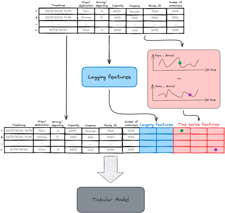
As you could have guessed, an ensemble of both tabular and time series models is used. The relation between rows (timestamps) is modeled on the one hand by so-called lagging features and on the other hand by carefully crafting time series using domain knowledge. Both the time series features, lagging features and existing ship schedule are concatenated, after which they are fed into a tabular model. The latter enables the relation between columns to be modeled. The process is illustrated in the figure below. Don’t worry, in the following paragraphs, each concept is elaborated.

Time series features

We could create a time series for each unique combination of variable values. However, this approach does not scale as the amount of features multiplies with each new variable and additionally it would lead to a sparse series. Nevertheless, it is very useful to generate them for only a subset of the variables that have an underlying meaning. For example, we can model the capacity over time of ships arriving from Peru, and do the same for ships arriving from China and the same for ships departing to China, ... you get the gist. Since the capacity is known upfront, we don’t need to forecast anything. Likewise, we can generate multiple time series the same way for the number of containers. Now, the time series is known up to the start of the forecast date, and we use an appropriate model to forecast one month into the future. Note that we have nicely modeled market supply (capacity) and demand (number of containers) in this way, at least for the port in question.

After generating the time series, we can use them to enrich the features of the ship entry. This is done by getting the appropriate time series, in the example corresponding to the right country and origin/destination, and picking the value at the timestamp of the entry (see the green and purple dots in the figure above). The attentive reader notices that we have made a time series forecast of the targets, and then used these to generate new features, which in turn is input into the tabular model to predict the target. This makes sense considering that the time series are created on a higher level, making the prediction task easier and viable for a time series model. These higher-level aggregations are now explicitly time-modeled and contain feature information that wasn’t there before for the tabular model.

There are multiple choices one can make for a time series model. In this case, a good fit with the properties of the data is the Prophet model by Meta. It can model yearly and weekly seasonality patterns, holidays of a lot of countries and long-term changing trends. It also trains fast, which is a requirement since a large number of time series are fitted.

Lagging features

In this timestamped data context, there is a strong seasonal effect at play meaning that the market has strong recurring patterns that can be yearly, quarterly, or weekly. We can exploit this by providing a direct link to the number of containers of the most similar ship entry on those time-lagged moments, hence the name. You can create your own definition of what ‘similar’ means in your context, e.g. filter first on company then on country etc. By using multiple lagging times, we generate some extra feature columns once again to aid the tabular model.

Tabular data modeling

Unlike the domain of images and text, transformers are not state-of-the-art in tabular data. In this field, gradient-boosted decision trees stand out. A good model choice is LightGBM, which is also made clear by the top winners in the popular M5 forecasting competition. It is a fast, proven method that has a relatively low number of tuning parameters.

Conclusion

Timestamped tabular data is a challenging format to make predictions for, without out-of-the-box solutions. Nevertheless, it can be of high value for businesses and opens the door to many use cases. By way of example, we showed some of the intricacies specific to this kind of data and worked out an approach to how to tackle such a problem.

The first step consists of providing a direct link to similar, historic data points, generating lagging features. In the second step, time series are crafted using domain knowledge after which these are forecasted into the future using an appropriate time series model. These generate in turn new features. In the end, they are all fed into a tabular data model.

How Radix can help

In our journey of assisting top companies with complex value chain challenges, we have been driving and experiencing firsthand the transformative power of AI integration. Some of our clients have already achieved significant improvements in planning efficiency and customer satisfaction.

The technique presented above is one of the tools that our framework uses to gain insights into demand variations, enabling enhanced planning workflows.

If you’re interested in a discussion or want to learn more, don’t hesitate to reach out!