Using Infrared Spectrum To Improve Night-Time Autonomous Driving

Are you a Machine Learning Engineer with a strong interest in Computer Vision? Are you interested to know how you can use information from sensors capturing light outside the visible spectrum to improve the quality of your (real-time!) object detection models? Then hold on tight, this article is for you!

In this blog post, we explain how we modified the architecture of YOLOv5 to perform object detection on multichannel images. Multichannel images are images containing information about the infrared (IR) and/or ultraviolet (UV) spectrum, on top of the classical RGB channels. We also show how we can take advantage of the pre-trained weights from the RGB space.

Leveraging information from the non-visible spectrum is useful in a wide range of applications such as the surveillance of industrial zonings, supply chain monitoring, detection of specific substances, etc. In this blog post, we illustrate our approach on a concrete autonomous driving dataset. We show that by leveraging IR channels, we significantly outperform traditional models using only the RGB channels.

Context

One of the main challenges in autonomous driving is the detection of the various “elements” that can be encountered on the road, from traffic lights to pedestrians, cars, bicycles, and other vehicles. Without real-time accurate detection, it is indeed impossible for the autonomous vehicle to make the right decisions, regardless of the algorithm. A bit like even a skillful human driver would have trouble driving blindfolded…

While traditional object detection algorithms work on traditional RGB images, capturing information from the visible spectrum, those typically do not capture detailed enough information in a dark environment. Infrared sensors, on the other hand, can better see at night but do not capture as many details during the day. By stacking the information from the visible and infrared spectrum, we get what is called a multichannel image. While RGB images are technically 3-channel images, multichannel here refers to the addition of one or several channels from the infrared spectrum, as illustrated in Figure 1.

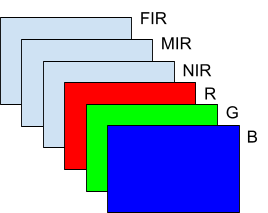
Figure 1. Representation of a multichannel image with 6 channels: RGB + 3 channels 
capturing information from the Near-, Mid- and Far-infrared spectrum respectively.

Though the human eye cannot see infrared light, it is clear that a well-designed machine learning model should be able to benefit from this additional information in order to make better predictions. Especially in poor lighting conditions or when the objects you are trying to detect are more easily detected in the IR or UV spectrum.

In the remainder of this blog post, we will briefly go through the different types of models that could be used to identify objects on an image (or a video) and explain why YOLOv5 is a great choice when inference speed is critical. We will then explain how the YOLOv5 architecture can be adapted to handle multichannel images, while still taking advantage of the pre-trained weights from the original RGB model. This challenge is also referred to as RGB to multichannel transfer learning.

Real-time object detection with YOLOv5

There are a plethora of model architectures that can be used to identify objects on an image, but they can essentially be split into 2 categories:

1. Object detection models. They provide as output a bounding box around the detected objects, and
2. Semantic segmentation models. They go even further by working at the pixel level, identifying exactly which pixels belong to which category of interest (+ the background for pixels that do not belong to any item we want to detect)

Bounding boxes are all we need

In our case, we were happy with a simple bounding box. In case you need semantic segmentation, make sure to have an appropriate dataset. Indeed, it is easy to automatically convert semantic segmentation labels to bounding box labels, but the opposite requires a significant amount of manual work.

Inference speed is critical

Another reason for sticking to bounding box object detection is that inference speed is crucial. We want to be able to process at least 4 images of size 6x320x320 (6 instead of 3 because we work with multichannel images) per second on a standard desktop equipped with a CPU (no GPU). The reason for this choice is that detecting traffic signs systematically too late is worse than occasionally failing at recognizing one. In other industrial applications, such as the monitoring of a fast production line, speed is more important than perfect accuracy. Given the time constraint, we want of course to make the most accurate predictions possible.

As they solve more complex tasks, semantic segmentation models generally run significantly slower than object detection ones. Of course, this is very architecture-dependent but stated in a non-scientific way, a fast object detection model will be faster than a fast semantic model.

With those criteria in mind, we went for YOLOv5, because this to the best of our knowledge one of the faster object detection algorithms. YOLO stands for You Only Look Once, and comes from the fact that the image is fed only once through the network that then makes all the predictions for the entire image. This is in contrast with other object detection models that successively examine sub-regions of the images to make predictions, hence requiring several passes through the network.

The table below shows the average inference time of 4 different models on a 320 by 320 RGB image. YOLOv5s, Faster-CNN and MobileNetv3 are all object detection models, while DeepLabv3 is a semantic segmentation architecture, based in this case on the EfficientNetv2 “backbone”. Without entering into the details, the backbone is the part of the model responsible for the features extraction, while the remainder of the architecture is responsible for converting those abstract features into actual predictions (e.g. bounding boxes or, in the case of DeepLabv3, semantic segmentation).

Table 1. Inference time for 320x320 RGB images on a conventional desktop computer using a CPU 
(2,3 GHz 8-Core Intel Core i9, 16GB).

Seeing in the night: leveraging multichannel images

At this point, we have identified that YOLOv5 is well suited for fast object detection applications, however, we still need to adapt it to make it work on multichannel images.

Since most of the available computer vision datasets consist of RGB images, the vast majority of the computer vision models have also been designed for - and trained on - such data. This makes it very easy to develop a computer vision model for a new application using transfer learning. Transfer learning consists in re-using a network that was trained on a “somehow similar task”, where a typically huge dataset was available, and then fine-tuning that network with a (typically small) dataset specific to the new application.

The challenge with multispectral images is the combination of the fact that there are far fewer datasets (and thus models) readily available, and that adapting an RGB model architecture to accommodate for the additional channels requires modifying at least the very first layer. This makes fine-tuning a priori much more difficult. Indeed, if we set the weights of the “pixels” from the infrared channels randomly, we will need a lot of data to retrain the model, as the randomness will propagate through all the subsequent layers (unlike in traditional transfer learning).

Custom weights initialization and dropout

To go around that issue, we initialize the new weights (corresponding to the new filters in the first convolutional layer) with the average of the pre-trained weights of the RGB channels in that layer. The intuition is that the object should have the same shapes in the visible (RGB) and infrared spaces. Therefore, the “feature detectors” that work in the RGB space should be a good starting point to extract features in the infrared space.

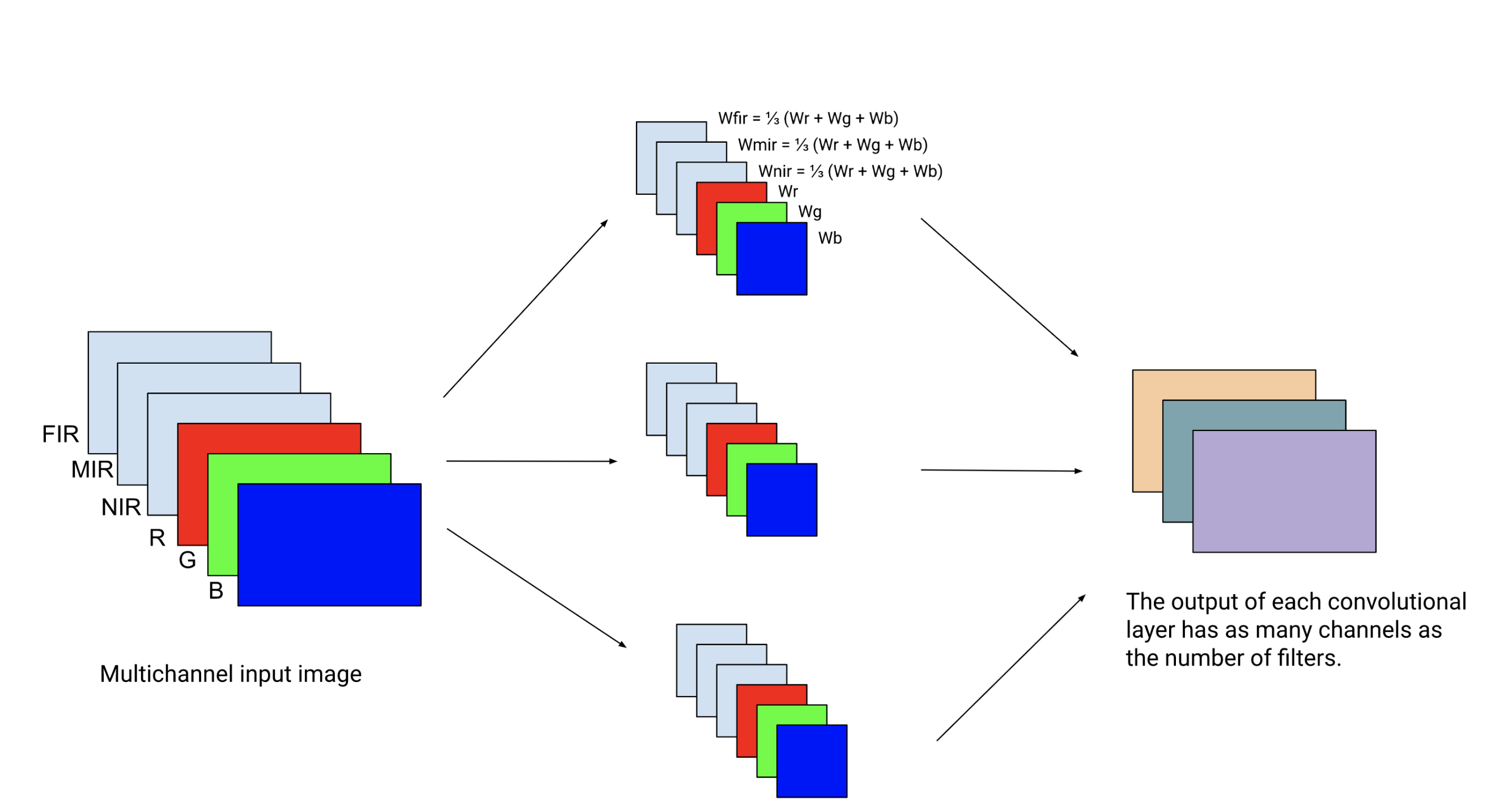Figure 2. Custom weights initialization of the additional channels in the first convolutional layer.
Here only 3 filters are represented). For each filter, the weights of the additional NIR, MIR, and
FIR channels are initialized as the average of the weights of the RGB channels.

While this alone was already working decently, we could further improve the predictions by also adding channels in the 2 layers after the input layer. Intuitively, this provides an increased learning capacity for the network, allowing to progressively “digest” the information from the extra input channels.

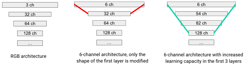Figure 3. Illustration of the increased learning capacity.

Finally, we also added a layer of 2D dropout after the first layer. At training time, this dropout acts like a blackout mask on an entire channel (leaving out for example the entire Red component for some training samples, removing the Blue component for other training samples, etc.). This helps the model to extract information from the new channels since it cannot always rely on the R, G and B channels during training. As always, dropout is deactivated at inference time. In other words, once the model is trained, it will use all the channels to make predictions.

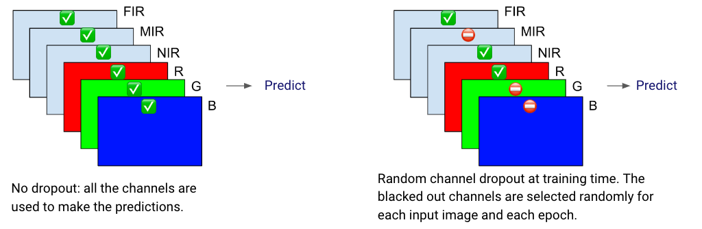Figure 4. Illustration of 2D dropout (aka channel dropout).

Results

We evaluated our methodology on the publicly available dataset used by T. Karakumi et al. in their paper "Multispectral Object Detection for Autonomous Vehicles'', The 25th Annual ACM International Conference on Multimedia (ACMMM 2017). This dataset contains 1446 images of shape 6x320x320. The 3 additional channels on top of RGB respectively correspond to near-infrared (NIR), mid-infrared (MIR), and far-infrared (FIR). The dataset has been split into training (75%), validation (10%), and test (15%) sets. All the results and performance figures reported below are coming from the test set.

Let’s look at a few examples!

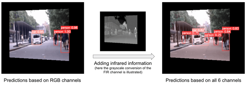
In this first example taken during the day, we can see that the model benefits from the extra channels to detect objects that were missed by the RGB-only model.

In this second example, taken at night, the benefit of the infrared channel is even more clear. We see that the RGB-only model wrongly detects a car stop and fails at recognizing the person (which is understandable as it is completely dark). 

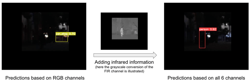
Those examples illustrate that the multichannel works better than the RGB-only model both during the day and during the night!

Can you put numbers on it?

The first metric that we look at is the precision-recall curve, also known as PR curve. This curve indicates the set of possible tradeoffs between precision and recall. Indeed, while both high precision (when the model detects a car, there is an actual car) and high recall (detect all cars) are wishable characteristics, there is always a tradeoff to find between the two. The more conservative you are about your predictions, the higher the precision, but the lower the recall, and vice-versa².

The area under the PR curve gives a good indication of how good the model is as it captures all the possible precision-recall tradeoffs that the model allows. In the graph below, we clearly see that the multichannel model outperforms the RGB model. In other words, for a fixed level of precision, say 80%, we can only retrieve 50% of the cars with the RGB model, while with the multichannel model exploiting the infrared information, we are able to retrieve more than 70% of the cars.

While this still might not sound so impressive, keep in mind that the dataset at our disposal is rather small. Increasing it or applying more advanced data augmentation techniques should boost the performance of both models, and the performance gap is actually expected to increase: the multichannel model would benefit the most from more data as it has more parameters to fine-tune.

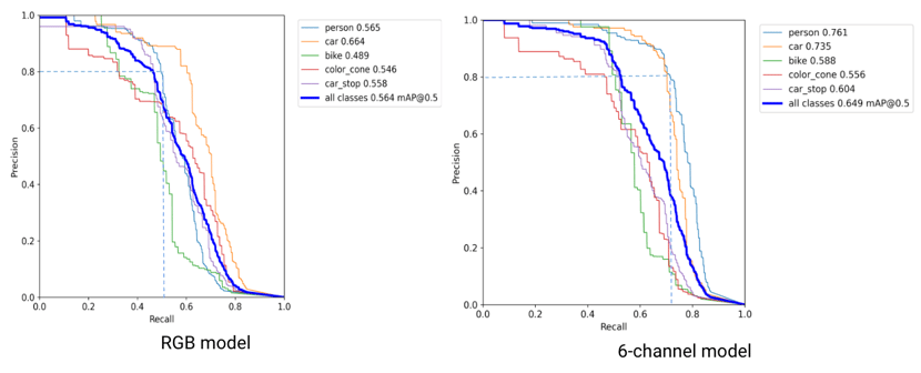Figure 5. Precision-recall curves. On the left, is the RGB model, and on the right the multichannel model.

The confusion matrix gives more insights into the precision of the model and also highlights the superiority of the model leveraging infrared information.

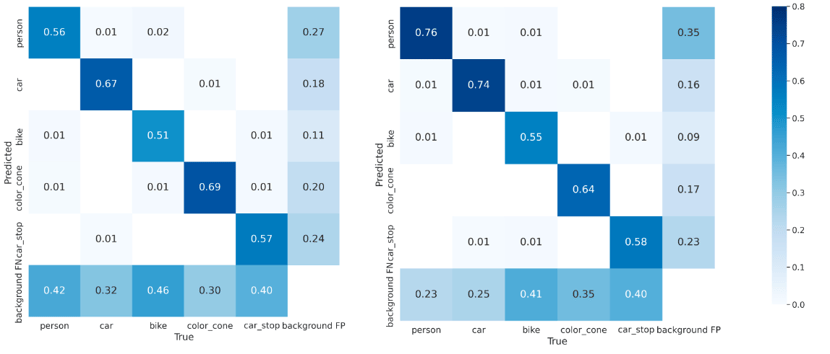Figure 6. Normalized confusion matrix. On the left, is the RGB model, and on the right the multichannel model.
The cell (i, j) represents the number of objects of class j predicted as class i, normalized
by the total number of objects of class i.

Conclusion

Traditional transfer learning is a well-established process that you can apply almost automatically whenever the input data of the new task has the same format as the one used by the original pre-trained model. However, when the model architecture needs to be adapted somewhere else than in the last layers, there was until now no standard way of applying transfer learning. While it requires a case-by-case analysis, we believe that our approach (increased network capacity in the first layers with custom weights initialization and 2D dropout) should work well in many RGB to multichannel transfer learning tasks. 

The range of applications is also very broad, including autonomous driving, surveillance of industrial zonings, supply chain monitoring, and detection of specific substances (chemical agents, …), to only cite a few examples.

Did you find it useful?

Feel free to chat with Mattia and Raphaël if you have questions!

¹ -There are different variants of the YOLOv5 architecture, respectively “nano”, “small”, “medium”, and “large” and “extra-large”, offering different tradeoffs in terms of speed and performance. We found the “small” version (YOLOv5s) to best suit our needs.

² - Note that in object detection, precision and recall are computed with respect to an “Intersection over Union” (IoU) metric measuring the overlap between the ground truth bounding boxes and the predicted bounding boxes. For our tests, we set that IoU threshold to 0.5, meaning that for a prediction to be considered correct, there must be an overlap of at least 50% with the ground truth. For more details, refer for example to this article.