Introduction

Operations research (OR) involves the development and application of analytical methods to improve decision-making and has been successfully employed in various domains including logistics and supply chain management, transportation, healthcare, finance, manufacturing, energy, etc. For instance, printing companies struggle with scheduling production jobs on a number of printing/labelling machines efficiently, while also respecting various constraints (e.g. machine maintenance) and objectives (minimize job lateness, startup time, etc.). At Radix, we have tackled this issue using advanced OR solvers to obtain feasible and fast schedules (see this blogpost for more info). However, implementing robust OR solutions presents challenges, including complex modelling, scaling to large-scale problems, and achieving real-time decision-making. For example, scheduling problems are often limited to tens or hundreds of jobs/machines, whereas industrial examples can reach over thousands of jobs/machines. 

In this blog post, we will provide a number of practical guidelines to keep in mind while you are implementing your OR problem using OR-Tools or any similar framework. We also provide notebooks with each guideline to illustrate how we practically obtained these results. Specifically:

• Keep your variables/constraints ratio low (colab)
• Try different modelling solutions (colab)
• Try different solver settings (colab)
• Add symmetry-breaking constraints (colab)
• Add hints (colab)

Let’s dive into it!

Keep your variables/constraints ratio low

A general rule of thumb for CP and MIP problems is to minimize the number of variables and maximize the amount of constraints. These two aspects essentially reduce the search space and consequently allow the solver to find feasible solutions faster. This can be obtained by thinking about which values are absolutely necessary, substitution, adding non-redundant constraints (e.g. based on heuristics), etc. As an illustration, we implemented three fundamental OR problems: a vanilla linear program (LP), a jobshop and a multi-knapsack problem. By scaling up these problems (e.g. increasing the number of variables or knapsacks), we can change the variable-to-constraints ratio and observe the resulting wall time required to solve these instances. The figure below shows the results.

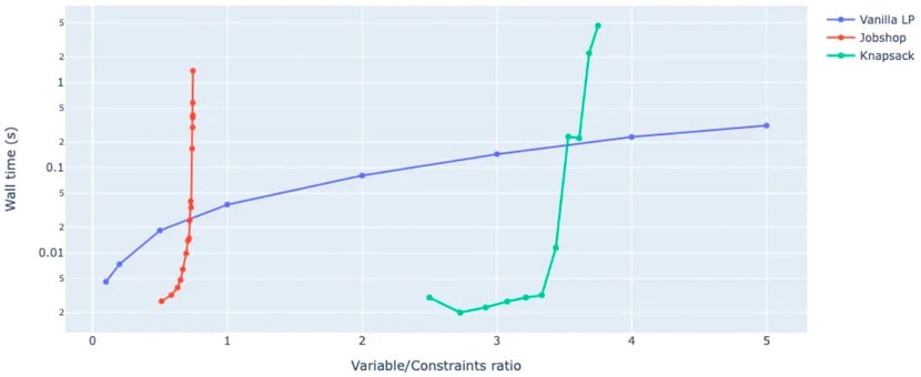
Figure 1. Variable/Constraint ratio versus average runtime for solving a vanilla LP, Jobshop and Knapsack Problem. Note the logarithmic scale on the y-axis.

The results clearly indicate an increasing trend. The more variables relative to constraints, the more processing time required to solve to optimality. More interestingly, this trend is different across the different problem types. Knapsack and in particular job shop problems tend to quickly explode as the variable/constraints ratio increases. This is much less the case for vanilla LP problems. This is due to more efficient solving algorithms for linear programming problems in comparison to mixed integer programming problems.

Try different modelling solutions

Operational research problems can often be solved using different model formulations. This may lead to different performances in terms of optimality for solving time. In general, there is no one-fits-all strategy, and it is a good idea to test various modelling solutions. Luckily, frameworks such as OR-Tools allow us to easily switch solvers or modelling strategies. We illustrate this with two examples.

Consider the travelling salesman problem (TSP). This can be formulated as a constraint programming (CP) or mixed integer programming (MIP) model. We implemented both approaches and evaluated the solving time as a function of the problem size. The results are shown in the following graph.

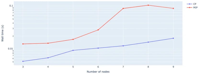
Figure 2. Average wall time (in s) for a TSP using CP and MIP formulation for various problem input sizes.

From this example, we can conclude that the CP solution is favourable over the MIP formulation. In general CP solvers tend to perform well on loosely constrained discrete programming problems such as the TSP and job shop problem. They typically perform worse on high-dimensional problems with lots of (particularly continuous) variables.

As a second example, we consider a generic linear problem with linear constraints, a linear minimization objective and integer variables. These problems can be solved to optimality using MIP solvers, or approximately through relaxation and LP solvers. The results are as follows:

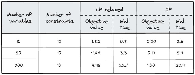
Figure 3. Performance of an LP relaxed and IP implementation in terms of objective value and wall time (in ms).

Due to the relaxation, the LP formulation fails to find an optimal (but fairly close) solution. The upside of the approach is that these solutions are found about an order of magnitude faster than the MIP solver. Consequently, there’s a compute/optimality trade-off here.

Try different solver settings

Solvers are rarely optimised to your specific use case. They typically come with a number of parameters that should be tuned to optimality. Even though out-of-the-box parameter settings may result in good performance, it can be worth the effort to look into these parameter settings.

Let’s consider a typical linear program. Using OR-Tools, it is fairly straightforward to obtain a solution, e.g. using the GLOP, Gurobi or PDLP solver. However, depending on the amount of variables, constraints, and sparsity of the problem, different solver settings can drastically improve performance. The figure below illustrates this on various LP instances (rows) using different settings of the GLOP, Gurobi and PDLP solvers (columns).

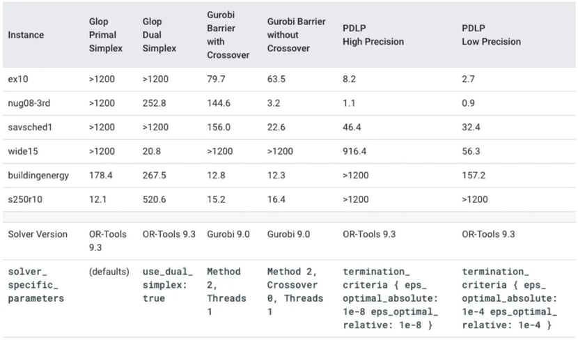
Figure 4. Required time (in seconds) to solve an LP instance to optimality using a specific solver configuration. Depending on the solver and parameter settings, solving time may be reduced by several orders of magnitude. Note that there is no real unique solver or parameter configuration that completely outperforms other cases. Source: https://developers.google.com/optimization/lp/lp_advanced

Alternatively, consider the 2D bin packing problem (BPP), which consists of a (relatively large) 2D container that should be filled with multiple (smaller) rectangular items. This problem is known to be NP-hard, but can be solved using the OR-Tools CP-SAT solver. As the scale of the problem (larger items and container) becomes larger, the problem becomes more and more challenging to solve. By adjusting problem-specific parameter settings such as use_energetic_reasoning_in_no_overlap_2d (use_er), use_timetabling_in_no_overlap_2d (use_tt) and use_pairwise_reasoning_in_no_overlap_2d (use_pr), significant gains may be obtained, as shown in the figure below. For a complete overview of all parameters in the CP-SAT solver, we refer to the OR-Tools repository.

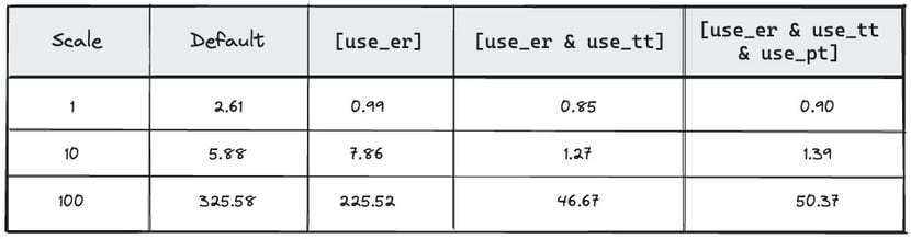
Figure 5. CP-SAT solving time (in seconds) for the 2D BPP problem. The problem (scale=1) corresponds to placing 24 randomly sized rectangles in a 40x15 container, whereas the default solver corresponds to the default CP-SAT solver. By switching on specific 2D-overlap-related parameters, we observe significant solving speed-ups (up to an order of magnitude).

Add symmetry-breaking constraints

What makes an optimization problem challenging is typically the size of the search space. By exploiting symmetries in the problem, it is possible to search this space in a much more efficient manner. Take for example the (v, b, r, k, l) balanced incomplete block-design (BIBD) problem, where we are trying to set up a binary v x b matrix such that the sum of the rows (resp. columns) equals r (resp. k) and the scalar product of every two rows equals l. This problem has applications in error control coding, cryptography, watermarking, communication & sensor networks, etc. and can be easily implemented with the CP solver in OR-Tools. For every (in)feasible solution, we can observe that swapping rows or columns does not change the feasibility of the solution. In general, any permutation of rows or columns results in an equivalent state. By ordering the rows and columns lexicographically, we allow the solver to skip many equivalent infeasible solutions. In the case of a BIBD, this has two benefits:

• If a solution exists, we are able to find a feasible solution faster. For example, for a (15, 15, 7, 7, 3) BIBD, a vanilla implementation can find a feasible solution in approximately 750 ms (average over 100 runs), whereas additional symmetry-breaking constraints allow us to find a solution within 250 ms.
• If a solution does not exist, we are able to show this much faster due to the drastically reduced search space. For example, for a (13, 13, 7, 7, 1) BIBD, a vanilla implementation can show this in approximately 72 s (average over 100 runs), whereas additional symmetry-breaking constraints allow us to do this within 50 ms!

There are some caveats when implementing symmetry-breaking solutions. They are advised whenever your goal is to find a feasible solution to the problem. For finding all solutions, symmetry-breaking constraints will only be able to give you a subset of the solutions. However, you could still generate the equivalent solutions based on the known symmetries. Perhaps the biggest challenge in implementing symmetry breaking is finding appropriate constraints for your type of symmetry. For symmetries on the variables (e.g. BIBDs, N-Queens, etc.), imposing a lexicographical ordering is usually a practical and efficient approach. For symmetries on the values (e.g. scene allocation), we can similarly impose a lexicographical ordering on the values instead of the variables.

Add hints

In many cases, we have a (rough) idea of what the solution of a combinatorial problem should look like. To this benefit, OR-Tools (and most similar packages) have a feature called hinting. This allows you to prioritize suggested values for specific variables throughout the search (model.AddHint(variable, value)). Note these values are not necessarily enforced! Therefore, it’s also possible to provide hints that may contain mistakes. To implement enforced value assignments, you will typically provide equality constraints (e.g. model.Add(variable == value)).

To illustrate the effect of adding hints, we tested them on the famous N-Queens problem. This problem consists of placing N queens (we chose N=32) on an NxN grid without violating the chess rules of placing a queen (i.e. no two queens on the same row, column or diagonal). A vanilla implementation solves this problem on average in about 90 ms. Usually, lots of hints have to be provided to obtain a significant solver speedup. However, by enforcing variable values, the problem can be solved in 39 ms. This shows the benefit of thinking about variables and their potential solution values.

Conclusion

In conclusion, operations research (OR) offers valuable tools for optimising decision-making across various domains, from logistics to finance. Implementing robust OR solutions can be challenging but is essential for achieving efficient results. This blog post has provided practical guidelines for implementing OR problems using frameworks like OR-Tools. For example: optimising the variables/constraints ratio, exploring different modelling approaches, fine-tuning solver settings, leveraging symmetry-breaking constraints, and providing hints to guide the search process. These guidelines empower practitioners to tackle complex OR problems effectively. While each problem may require a unique approach, considering these principles can enhance the efficiency and effectiveness of OR implementations.

Interested in more practical tools for tips and know-how on OR-Tools, have a look at this cheat sheet written by Dominik Krupke, or these recipes for OR-Tools provided by Xiang Chen!